Session 4 – Object-Oriented Programming and Modeling Libraries

Session Overview

In this session, we’ll cover object-oriented programming and how it applies to modeling and analysis workflows in Python.

Topics:

• Intro to OOP and how it makes modeling in Python different from R
• Building and extending classes using inheritance and mixins
• Applying OOP to machine learning through demos with scikit-learn and PyTorch
• Creating and using models
• Plotting data with plotnine and seaborn

This is the last session of the intro to python workshops. There will be a brief ‘homework’ that covers the topics in this session. We may not have time to finish it in class, but there is a solutions guide on our github repo.

Introduction

Why Python Feels Different from R 🐍

R: Built by Statisticians

• Designed for statistical analysis

Python: General-Purpose Language

• Designed for many domains, not just statistics

• Workflows are primarily functional:
  • pass data into functions
    
  • get back results (usually without modifying the original object)

• Leans heavily on object-oriented programming:
  • Some methods modify objects in-place, rather than returning new ones

• Pipes (|>, %>%) chain operations

• Method chaining (.fit().predict())

• Excels at:
  • clean model outputs, tables and high-quality visualizations

• Excels at:
  • machine learning & deep learning (scikit-learn, PyTorch)
    
  • image, genomic, and single-cell analysis
    
  • software, automation, and tooling

💡 You’ve already been using this style in Sessions 2 and 3 — creating objects (lists, DataFrames) and calling methods like .append() or .sort_values(). Note: Tools like reticulate and rpy2 allow R and Python to coexist in the same project, but that’s beyond the scope of this course.

As Yufei mentioned in session 1, R and Python have different flavors of coding. R was fundamentally designed for statistics while Python is a more general-purpose language.

Core OOP Principles in Python - Objects, classes and methods

Classes and objects

• An object (instance) has attributes (data) and methods (behaviors)

• A class is a blueprint for objects
  • The class defines what attributes and methods an object will have

• Use type(obj) and isinstance(obj, Class) to check the class of an object

Before we talk about Object-Oriented programming, let’s first define classes and objects. An object is a self-contained unit in code that holds data (attributes) and behaviors (methods) that work on that data. In code, methods are like functions that are attached to an object. Classes are blueprints for objects that define the attributes and methods available for an object of that class. We can check the class of an object using type or isinstance.

Core OOP Principles in Python - OOP Paradigm

Python’s object-oriented design builds on a few key principles of how objects behave:

1. Encapsulation — Data and behaviors live together

   • Attributes store data, methods define behaviors

2. Inheritance — New classes reuse existing functionality

   • Classes can inherit attributes and methods from parent classes.
     
   • Avoids re-writing shared logic

3. Abstraction — Same interface hides complexity

   • Interact with what things do, not how they work.

4. Polymorphism (Duck Typing) — Different objects with the same methods can be used interchangeably

   • This makes it easy to switch between models with minimal code adjustment (assuming similar api)

Why OOP Matters for Python Modeling

In Python modeling frameworks:

• Models are objects (class instances)
  
• They have methods like .fit(), .predict(), .score()
  
• Learned parameters (coefficients, weights, layers) live in attributes

This consistent object-oriented API makes it easy to swap models with minimal code changes.

Examples of Python modeling libraries:

• scikit-learn — general ML (classification, regression)
  
• xgboost — gradient boosting
  
• scikit-survival — survival models using sklearn API
  
• statsmodels — statistical models with R-like outputs
  
• scvi-tools — single-cell models
  
• PyTorch / TensorFlow — deep learning frameworks

Understanding classes is ESPECIALLY important for using PyTorch and TensorFlow!

• In Python, modeling libraries make models objects rather than simple functions.
  
• Models combine both the code that defines how predictions are made and the data the model has learned during training.
  
• After .fit(), attributes like .coef_, .classes_, or learned weights in a neural network store the fitted state directly on the model object.

Consistent interface across libraries

• The methods .fit(), .predict(), and .score() behave similarly across many model types, even though the internals differ.
  
• This consistency reduces cognitive load and lets you swap models (e.g., from logistic regression to random forest) without changing your workflow.

Library examples

• scikit-learn: classic ML models with a predictable API.
  
• xgboost: gradient boosting with same pattern for .fit()/.predict().
  
• scikit-survival: survival analysis models built on sklearn conventions.
  
• statsmodels: statistical modeling with output more like R; still object-oriented but less uniform.
  
• scvi-tools: variational inference models for single-cell data.
  
• PyTorch and TensorFlow: neural network tools where you define your own model classes, but they follow the same idea — methods and attributes attached to objects.

Key takeaway

• Think of a model as a container of behavior (methods) and state (attributes).
  
• This object-oriented pattern underlies many Python modeling workflows and makes advanced use (like wrapping PyTorch models to act like sklearn models) intuitive.
  

Bonus: Python Modeling Libraries — Tutorials & Docs

• scikit-learn (ML basics) — official API & guide (general modeling) https://scikit-learn.org/stable/user_guide.html

• xgboost (gradient boosting) — official documentation with examples/tutorials https://xgboost.readthedocs.io/ (look under Tutorials)

• scvi-tools (probabilistic single-cell modeling) — user guide + tutorials https://docs.scvi-tools.org/en/stable/ (Tutorials section)

• scikit-survival (survival analysis with sklearn API) — user guide & intro notebook https://scikit-survival.readthedocs.io/en/stable/ (00-introduction tutorial)

• statsmodels (statistical modeling & inference) — getting started & examples https://www.statsmodels.org/stable/gettingstarted.html Also see: https://www.statsmodels.org/stable/examples/index.html

These are some links to tutorials for the packages I mentioned.

OOP In Practice: Creating Classes

• To really understand how object-oriented programming works, let’s create some simple classes and see how they behave.
• While the following examples are really simple, they showcase the same concepts used when designing the kinds of Python libraries you’ll be using
• If you work with PyTorch or TensorFlow you will likely be making model classes yourself

Base Classes

A base class serves as a template for creating objects. Other classes can inherit from it to reuse its attributes and methods.

Classes are defined using the class keyword, and their structure is specified using an __init__() method for initialization.

Define a Dog with attributes (data) and methods (behaviors).
* special or “dunder” methods (short for double underscore) define how objects behave in certain contexts.

class Dog: ## begin class definition
    def __init__(self, name, breed): ## define init method
        self.name = name ## add attributes
        self.breed = breed

    def speak(self): ## add methods
        return f"{self.name} says woof!"

    def __str__(self): # __str__(self) tells python what to display when an object is printed
        return f"Our dog {self.name}"

    def __repr__(self): # add representation to display when dog is called in console
        return f"Dog(name={self.name!r}, breed={self.breed!r})"

A base class serves as a template for creating objects and other classes can inherit its attributes and methods. Classes are defined using the ‘class’ keyword and their structure is specified using an init method for initialization.

For example, we can define a class called Dog and give it attributes that store data about a given dog and methods that represent behaviors an object of the Dog class can perform.

First we will define our init method, which sets up the structure for objects of the dog class. The parameters here (name and breed) can be stored as attributes. The speak method here defines the speech behavior for the dog and returns a string, that changes based on the value stored in the ‘name’ attribute.

We can also define our str and repr methods which tell python what to do when an object is printed (str) or called in console (repr). These methods are useful for displaying information about objects at a glance. We will see an interesting example of a repr method later on.

Creating a dog

Creating an instance of the Dog class lets us model a particular dog:

buddy = Dog("Buddy", "Golden Retriever")
print(f"Buddy is an object of class {type(buddy)}")

Buddy is an object of class <class '__main__.Dog'>

• Set value of attributes [name and breed] -> stored as part of buddy
• buddy can use any Dog class methods

## if we want to see what kind of dog our dog is
## we can call buddy's attributes
print(f"Our dog {buddy.name} is a {buddy.breed}.")

## we can also call any Dog methods
print(buddy.speak())  

## including special methods
buddy ## displays what was in the __repr__() method

Our dog Buddy is a Golden Retriever.
Buddy says woof!

Dog(name='Buddy', breed='Golden Retriever')

Note: For python methods, the self argument is assumed to be passed and therefore we do not put anything in the parentheses when calling .speak(). For attributes, we do not put () at all.

If we want to model a particular dog, we create an instance of the dog class. The arguments we pass to Dog set the name and breed of the dog.

If we want to prove that buddy is an object of class dog, we can use type(buddy).

Once we create buddy, we can use any attributes or methods defined in the dog class.

Derived (Child) Classes

Derived/child classes build on base classes using the principle of inheritence.

Now that we have a Dog class, we can build on it to create a specialized GuardDog class.

class GuardDog(Dog):  # GuardDog inherits from Dog
    def __init__(self, name, breed, training_level): ## in addition to name and breed, we can 
        # define a training level. 
        # Call the parent (Dog) class's __init__ method
        super().__init__(name, breed)
        self.training_level = training_level  # New attribute for GuardDog that stores the 
        # training level for the dog

    def guard(self): ## checks if the training level is > 5 and if not says train more
        if self.training_level > 5:
            return f"{self.name} is guarding the house!"
        else:
            return f"{self.name} needs more training before guarding."
    
    def train(self): # modifies the training_level attribute to increase the dog's training level
        self.training_level = self.training_level + 1
        return f"Training {self.name}. {self.name}'s training level is now {self.training_level}"

# Creating an instance of GuardDog
rex = GuardDog("Rex", "German Shepherd", training_level= 5)

Derived or child classes build on base classes using the principle of inheritence. This helps us build more specialized classes without having to start from scratch.

If we want to make a new guardDog class, we can start by inheriting the attributes and methods of the dog class by putting ‘Dog’ in the parentheses here.

When we define our init method, we can first call the parent class’s init method to assign the dog’s name and breed. We can also add an additional attribute that stores the dog’s training level.

Because of inheritence, guarddogs also have the speak method, but we can also give them new methods like guard and train. The guard method, like the speak method earlier, just returns a value. However, the train method actually modifies the training_level attribute of the object in-place. This means that, if we want to train a guarddog, we do not have to assign the trained dog to a new variable to preserve the trained state.

Let’s make an instance of guarddog called rex and we can see how this works.

rex has all of the methods/attributes introduced in the Dog class as well as the new GuardDog class.

Using methods from the base class:

print(rex.speak())
rex

Rex says woof!

Dog(name='Rex', breed='German Shepherd')

This is the power of inheritance—we don’t have to rewrite everything from scratch!

Using a method from the child class:

print(f"{rex.name}'s training level is {rex.training_level}.")
print(rex.guard()) 

Rex's training level is 5.
Rex needs more training before guarding.

Of course we can use the speak() and repr() methods that we defined for the dog class. We can also use the training method that we just defined. adv

to successfully guard, a rex needs a training level greater than 5. Currently his level is 5, so he needs more training before guarding.

Unlike standalone functions, methods in Python often update objects in-place— meaning they modify the object itself rather than returning a new one.

We can use the .train() method to increase rex’s training level.

print(rex.train())

Training Rex. Rex's training level is now 6

Be Careful!!!

Calling rex.train() within a print statement still updates rex’s training level. If we were to do this instead:

rex.train()
print(rex.train())

it would train rex twice!

Now if we check,

print(f"{rex.name}'s training level is {rex.training_level}.")
print(rex.guard()) 

Rex's training level is 6.
Rex is guarding the house!

As with Rex, child classes inherit all attributes (.name and .breed) and methods (.speak() __repr__()) from parent classes. They can also have new methods (.train()) or re-define methods from the parent class.

Unlike standalone functions, methods like train() update objects in-place instead of returning a new object. This allows us to increase rex’s training level without storing rex to a new variable.

Please note that even though we’re calling rex.train() within a print statement, it still updates rex’s training level!

After training rex once, we can see that his training level is sufficient to allow him to guard! adv

as we saw with rex, child classes inherit all attributes and methods from their parent classes, but they can also have new ones.

Mixins

A mixin is a special kind of class designed to add functionality to another class. Unlike base classes, mixins aren’t used alone.

For example, scikit-learn uses mixins like:
- sklearn.base.ClassifierMixin (adds classifier-specific methods)
- sklearn.base.RegressorMixin (adds regression-specific methods)

which it adds to the BaseEstimator class to add functionality.

To finish up our dog example, we are going to define a mixin class that adds learning tricks to the base Dog class and use it to create a new class called SmartDog.

Mixins area special kind of class that take advantage of the inheritence property to add functionality to other classes without needing to re-define the initial class structure. Unlike base classes, mixins are not useful on their own.

Some examples of mixin classes are ClassifierMixin and RegressorMixin from scikit learn, which add functionality to the BaseEstimator class. To finish up our dog example, we are going to define a mixin class that adds learning tricks to the base Dog class and use it to create a new class called SmartDog.

When creating a mixin class, we let the other base classes carry most of the initialization

class TrickMixin: ## mixin that will let us teach a dog tricks
    def __init__(self, *args, **kwargs):
        super().__init__(*args, **kwargs)  # Ensures proper initialization in multi inheritance
        self.tricks = []  # Add attribute to store tricks

## add trick methods
    def learn_trick(self, trick):
        """Teaches the dog a new trick."""
        if trick not in self.tricks:
            self.tricks.append(trick)
            return f"{self.name} learned a new trick: {trick}!"
        return f"{self.name} already knows {trick}!"

    def perform_tricks(self):
        """Returns a list of tricks the dog knows."""
        if self.tricks:
            return f"{self.name} can perform: {', '.join(self.tricks)}."
        return f"{self.name} hasn't learned any tricks yet."

## note: the TrickMixin class is not a standalone class!

When we create a mixin class, we let the base class carry most of the initialization.

A mixin class can add both attributes adv and methods, and it can potentially work with multiple base classes.

By including both Dog and TrickMixin as base classes, we give objects of class SmartDog the ability to speak and learn tricks! This is how libraries like sklearn turn a base estimator into a classifier/regressor without rewriting everything!

class SmartDog(Dog, TrickMixin):
    def __init__(self, name, breed):
        super().__init__(name, breed)  # Initialize Dog class
        TrickMixin.__init__(self)  # Initialize TrickMixin separately

# a SmartDog object can use methods from both parent object `Dog` and mixin `TrickMixin`.
my_smart_dog = SmartDog("Buddy", "Border Collie")
print(my_smart_dog.speak()) 

Buddy says woof!

print(my_smart_dog.learn_trick("Sit"))  
print(my_smart_dog.learn_trick("Roll Over")) 
print(my_smart_dog.learn_trick("Sit"))  

Buddy learned a new trick: Sit!
Buddy learned a new trick: Roll Over!
Buddy already knows Sit!

print(my_smart_dog.perform_tricks()) 

Buddy can perform: Sit, Roll Over.

By including both dog and trickmixin as base classes, we give smartdog objects the ability to ‘speak’ and learn tricks. -adv through-

Duck Typing

🦆 “If it quacks like a duck and walks like a duck, it’s a duck.” 🦆

Python’s duck typing makes our lives a lot easier, and is one of the main benefits of methods over functions:

• Inheritence - objects inherit methods from base classes
• Repurposing old code - methods by the same name work the same for different model types
• Use methods without checking types - methods are assumed to work on the object they’re attached to

We can demonstrate duck typing by defining two new base classes that are different than Dog but also have a speak() method.

class Human:
    def __init__(self, name):
        self.name = name

    def speak(self):
        return f"{self.name} says hello!"

class Parrot:
    def __init__(self, name):
        self.name = name

    def speak(self):
        return f"{self.name} says squawk!"

In my opinion python’s ducktyping makes our lives a lot easier and is a good reason to use methods when possible. Duck typing makes it easy to repurpose old code with few changes - because methods by the same name work the same for different model types, even if the underlying method code is very different. Models from the same package likely share a base class, or at least can be expected to have a similar API. Duck typing also stops us from having to check object types before performing operations as methods are assumed to work on the object they’re attached to.

We can demonstrate this by defining two new base classes that are different than dog but also have a speak method. -adv-

The human and parrot class here both have a speak method and a name attribute like the dog class.

Duck Typing in Action

Even though Dog, Human and Parrot are entirely different classes…

def call_speaker(obj):
    print(obj.speak()) ## No object checking needed here!

call_speaker(Dog("Fido", "Labrador"))
call_speaker(Human("Alice"))
call_speaker(Parrot("Polly"))

Fido says woof!
Alice says hello!
Polly says squawk!

They all implement .speak(), so Python treats them the same!

While our dog example was very simple, this is the same way that model classes work in python!

Warning

With duck typing, Python lets us use methods without breaking. It does not mean that any given method is correct to use in all cases, or that all similar objects will have the same methods.

Even though the three classes are different, we can still write a function that performs ‘obj.speak()’ and pass in any object with this method without having to worry about the object’s class. This will be true of future objects containing a speak method as well. If we used a function for ‘speak’ instead of a method, there would be no guarantee that call_speaker would work for a new object of a non-specified type.

Recap: Key Benefits of OOP in Machine Learning

1. Encapsulation – Models store parameters and methods inside a single object.
   
2. Inheritance – New models can build on base models, reusing existing functionality.
   
3. Abstraction – .fit() should work as expected, regardless of complexity of underlying implimentation.
4. Polymorphism (Duck Typing) – Different models share the same method names (.fit(), .predict()), making them easy to use interchangeably, particularly in analysis pipelines.

Understanding base classes and mixins is especially important when working with deep learning frameworks like PyTorch and TensorFlow, which require us to create our own model classes.

To recap: python’s oject oriented nature has some notable benefits for modeling and machine learning.

Part B - Demo Projects

Apply knowledge of OOP to modeling using scikit-learn and pytorch

🐧 Mini Project: Classifying Penguins with scikit-learn and pytorch

Now that you understand classes and data structures in Python, let’s apply that knowledge to classify penguin species using two features:

• bill_length_mm
• bill_depth_mm

We’ll explore:

• Unsupervised learning with K-Means clustering (model doesn’t ‘know’ y)
• Supervised learning with a Neural Network classifier (model trained w/ y information)

All scikit-learn models are designed to have

Common Methods:

• .fit() — Train the model
• .predict() — Make predictions

Common Attributes:

• .classes_, .n_clusters_, etc.

This is true of the scikit-survival package too!

For the rest of this session, we’ll be going through 2 mini projects to classify penguin species using bill length and bill depth using kmeans from scikit-learn and a Neural Network built with PyTorch. In terms of API, all sklearn models are designed to have common methods like fit and predict and have some attributes like .classes_ or .n_clusters_ that store information needed to specify the model.

We’ll follow a fairly typical analysis workflow including data visualization, pre-model preparation, model fitting and evaluation.

Import Libraries

Before any analysis, we must import the necessary libraries.

For large libraries like scikit-learn, PyTorch, or TensorFlow, we usually do not import the entire package. Instead, we selectively import the classes and functions we need.

Classes
- StandardScaler — for feature scaling
- KMeans — for unsupervised clustering

🔤 Naming Tip:
- CamelCase = Classes
- snake_case = Functions

Functions
- train_test_split() — to split data into training and test sets
- accuracy_score() — to evaluate classification accuracy
- classification_report() — to print precision, recall, F1 (balance of precision and recall), Support (number of true instances per class) - adjusted_rand_score() — to evaluate clustering performance

Our first step is always to import any necessary libraries - but in this case, we will import specific classes and functions we plan to use. For our classes, we’ll need standardscaler as well as our two model classes. We’ll also import some useful functions for splitting our dataset into training/test sets and computing classification scores.

A quick tip: for most python libraries, classes use CamelCase and functions use snake_case.

Import Libraries

## imports
import pandas as pd
import numpy as np

from plotnine import *
import seaborn as sns
import matplotlib.pyplot as plt

from great_tables import GT

## sklearn & PyTorch imports

## import classes
from sklearn.preprocessing import StandardScaler 
from sklearn.cluster import KMeans

## import functions
from sklearn.model_selection import train_test_split
from sklearn.metrics import accuracy_score, classification_report, adjusted_rand_score

## Pytorch Imports
import torch
import torch.nn as nn
import torch.optim as optim
from torch.utils.data import TensorDataset, DataLoader

Data Preparation

# Load the Penguins dataset
penguins = sns.load_dataset("penguins").dropna()

# Make a summary table for the penguins dataset, grouping by species. 
summary_table = penguins.groupby("species").agg({
    "bill_length_mm": ["mean", "std", "min", "max"],
    "bill_depth_mm": ["mean", "std", "min", "max"],
    "sex": lambda x: x.value_counts().to_dict()  # Count of males and females
})

# Round numeric values to 1 decimal place (excluding the 'sex' column)
for col in summary_table.columns:
    if summary_table[col].dtype in [float, int]:
        summary_table[col] = summary_table[col].round(1)

# Display the result
display(summary_table)

	bill_length_mm				bill_depth_mm				sex
	mean	std	min	max	mean	std	min	max	<lambda>
species
Adelie	38.8	2.7	32.1	46.0	18.3	1.2	15.5	21.5	{'Male': 73, 'Female': 73}
Chinstrap	48.8	3.3	40.9	58.0	18.4	1.1	16.4	20.8	{'Female': 34, 'Male': 34}
Gentoo	47.6	3.1	40.9	59.6	15.0	1.0	13.1	17.3	{'Male': 61, 'Female': 58}

We’re using the penguins dataset from the seaborn package, so we can use the load_dataset function to get that. We can also drop any na values with the .dropna() method.

We can then make a quick summary table for the dataset using some of the methods covered last session.

Data Visualization

For visualization: use either seaborn or plotnine. plotnine mirrors ggplot2 syntax from R and is great for layered grammar-of-graphics plots, while seaborn is more convienient for multiple plots on the same figure.

Plotting with Plotnine vs Seaborn

Plotnine (like ggplot2 in R)
The biggest differences between plotnine and ggplot2 syntax are:

• With plotnine the whole call is wrapped in () parentheses
• Variables are called with strings ("" are needed!)
• If you don’t use from plotnine import *, you will need to import each individual function you plan to use!

Seaborn (base matplotlib + enhancements)

• Designed for quick, polished plots
• Works well with pandas DataFrames or NumPy arrays
• Integrates with matplotlib for customization
• Good for things like decision boundaries or heatmaps
• Harder to customize than plotnine plots

To visually check out our data, we can use either plotnine (which is designed to work like ggplot) or seaborn (base matplotlib + enhancements). For single plots, plotnine can be more convenient but seaborn has better support for putting multiple plots on the same figure.

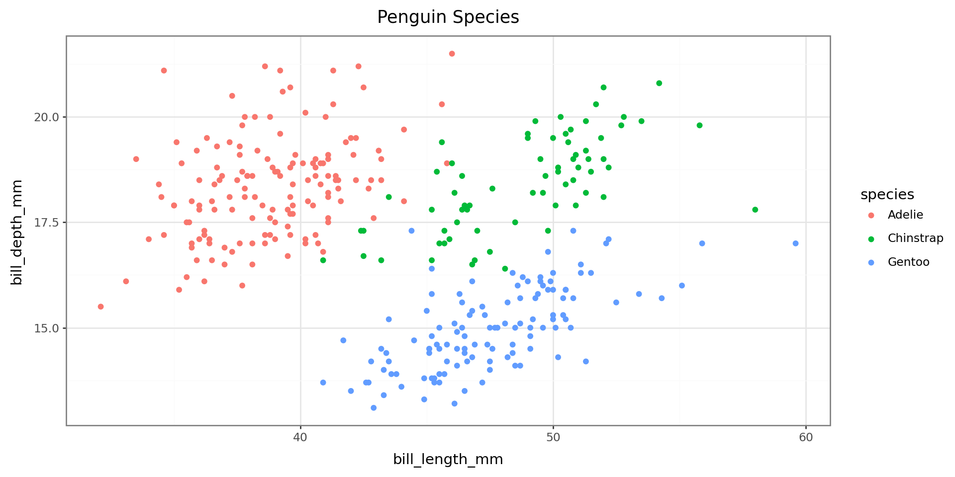
Scatterplot with plotnine

To take a look at the distribution of our species by bill length and bill depth before clustering…

plot1 = (ggplot(penguins, aes(x="bill_length_mm", y="bill_depth_mm", color="species"))
 + geom_point()
 + ggtitle("Penguin Species")
 + theme_bw())

display(plot1)

To plot our bill length and depth with plotnine, we can pretty much use ggplot syntax, but wrap the whole statement in parentheses. However, our variable names need to be entered as strings.

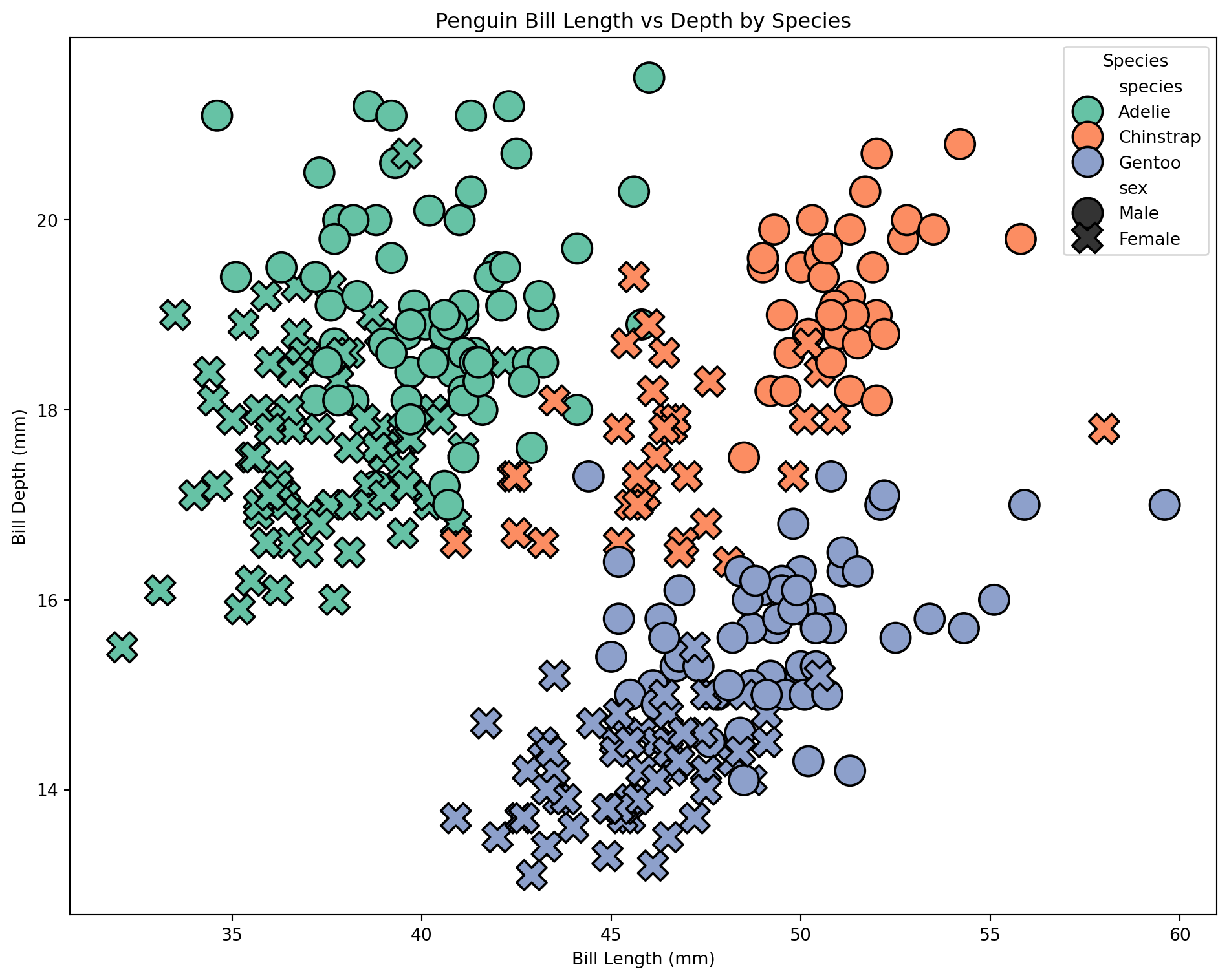
Scatterplot with seaborn

We can make a similar plot in seaborn. This time, let’s include sex by setting the point style

# Create the figure and axes obects
fig, ax = plt.subplots(figsize=(10, 8))

# Create a plot 
sns.scatterplot(
    data=penguins, x="bill_length_mm", y="bill_depth_mm",
    hue="species", ## hue = fill
    style="sex",  ## style = style of dots
    palette="Set2", ## sets color pallet
    edgecolor="black", s=300, ## line color and point size 
    ax=ax              ## Draw plot on ax      
)

# Use methods on ax to set title, labels
ax.set_title("Penguin Bill Length vs Depth by Species")
ax.set_xlabel("Bill Length (mm)")
ax.set_ylabel("Bill Depth (mm)")
ax.legend(title="Species")

# Plot the figure
fig.tight_layout() 
#fig.show() -> if not in interactive

If we want to do the same thing in seaborn, we can use sns.scatterplot() directly (which doesn’t save the figure to a variable), or we can create figure and axis objects first and then draw the plot on the created axis. We then use methods on the axis object to set the titles and labels.

Because we are working in an interactive notebook, we don’t have to explicitly use plt.plot() to display the figure.

Scatterplot with seaborn

Scaling the data - Understanding the Standard Scaler class

For our clustering to work well, the predictors should be on the same scale. To achieve this, we use an instance of the StandardScaler class.

class sklearn.preprocessing.StandardScaler(*, copy=True, with_mean=True, with_std=True)

Parameters are supplied by user
- copy, with_mean, with_std

Attributes contain the data of the object
- scale_: scaling factor
- mean_: mean value for each feature
- var_: variance for each feature
- n_features_in_: number of features seen during fit
- n_samples_seen: number of samples processed for each feature

Methods describe the behaviors of the object and/or modify its attributes
- fit(X): computes mean and std used for scaling and ‘fits’ scaler to data X
- transform(X): performs standardization by centering and scaling X with fitted scaler
- fit_transform(X): does both

For our clustering to work well, we typically want to put all of the predictors on the same scale. We can do this using an instance of the StandardScaler class.

We supply the parameters that dictate the behavior of the scaler at instantiation. The new scaler object has attributes that contain the information the object needs to perform its functions, like the scaling factor, feature means and variances, etc.

It also has methods that can modify its attributes, like the fit method, which calculates the mean and variance used for scaling based on data X, and the tranform method which uses the calculated values to scale X.

For convenience there is also the fit_transform() method that does both to the same data. When we look at our model classes, we’ll see that they also have fit methods.

Scaling Data

# Selecting features for clustering -> let's just use bill length and bill depth.
X = penguins[["bill_length_mm", "bill_depth_mm"]]
y = penguins["species"]

# Standardizing the features for better clustering performance
scaler = StandardScaler() ## create instance of StandardScaler
X_scaled = scaler.fit_transform(X) 

Original vs Scaled Features
Feature	Original		Scaled
	Bill Length	Bill Depth	Bill Length	Bill Depth
mean	44	17	0	0
std	5	2	1	1

## Make X_scaled a pandas df
X_scaled_df = pd.DataFrame(X_scaled, columns=X.columns)

# Compute summary statistics and round to 2 sig figs
original_stats = X.agg(["mean", "std"])
scaled_stats = X_scaled_df.agg(["mean", "std"])

# Combine into a single table with renamed columns
summary_table = pd.concat([original_stats, scaled_stats], axis=1)
summary_table.columns = ["Bill_Length_o", "Bill_Depth_o", "Bill_Length_s", "Bill_Depth_s"]
summary_table.index.name = "Feature"

# Display nicely with great_tables
(
    GT(summary_table.reset_index()).tab_header("Original vs Scaled Features")
    .fmt_number(columns =  ["Bill_Length_o", "Bill_Depth_o", "Bill_Length_s", "Bill_Depth_s"], decimals=0)
    .tab_spanner(label="Original", columns=["Bill_Length_o", "Bill_Depth_o"])
    .tab_spanner(label="Scaled", columns=["Bill_Length_s", "Bill_Depth_s"])
    .cols_label(Bill_Length_o = "Bill Length", Bill_Depth_o = "Bill Depth", Bill_Length_s = "Bill Length", Bill_Depth_s = "Bill Depth")
    .tab_options(table_font_size = 16)
)

To keep things simple, we will just subset the penguins dataset and keep only bill length and depth for our X dataframe. For y, we’ll grab the species as a pandas series.

The next step is to create the scaler object and use fit_transform to both fit the scaler to X and return the transformed X matrix. One of the nice things about using a scaler object rather than a function is that the object saves the scaling parameters so we can reuse them later.

This table here just shows how the mean and standard deviation change between the original and scaled features. It was made with great_tables and the code is included below.

Understanding the KMeans model class

class sklearn.cluster.KMeans(n_clusters=8, *, init='k-means++', n_init='auto', max_iter=300, 
tol=0.0001, verbose=0, random_state=None, copy_x=True, algorithm='lloyd')

Parameters: Set by user at time of instantiation
- n_clusters, max_iter, algorithm

Attributes: Store object data
- cluster_centers_: stores coordinates of cluster centers
- labels_: stores labels of each point - n_iter_: number of iterations run (will be changed during method run)
- n_features_in and feature_names_in_: store info about features seen during fit

Methods: Define object behaviors
- fit(X): fits model to data X - predict(X): predicts closest cluster each sample in X belongs to
- transform(X): transforms X to cluster-distance space

Now that we have our scaled data, the next step is to create and fit the kmeans model. Like the standardScaler class earlier, we have parameters set by the user. This is where we would specify the number of clusters we want, etc.

There are also attributes that store information like the location of cluster centers and the cluster labels associated with each point. These attributes are set by the fit method and wont exist for a model that has not been fit yet.

And we have the fit and tranasform methods like the scaler class. We also get a predict method that lets us predict cluster labels for any new input data in the same cluster-space.

Create model

## Choosing 3 clusters b/c we have 3 species
kmeans = KMeans(n_clusters=3, random_state=42) ## make an instance of the K means class
kmeans

KMeans(n_clusters=3, random_state=42)

In a Jupyter environment, please rerun this cell to show the HTML representation or trust the notebook.
On GitHub, the HTML representation is unable to render, please try loading this page with nbviewer.org.

Fit model to data

## the fit
penguins["kmeans_cluster"] = kmeans.fit_predict(X_scaled)

## now that we fit the model, we should have cluster centers
print("Coordinates of cluster centers:", kmeans.cluster_centers_)

## shows that model is fitted
kmeans

Coordinates of cluster centers: [[-0.95023997  0.55393493]
 [ 0.58644397 -1.09805504]
 [ 1.0886843   0.79503579]]

KMeans(n_clusters=3, random_state=42)

In a Jupyter environment, please rerun this cell to show the HTML representation or trust the notebook.
On GitHub, the HTML representation is unable to render, please try loading this page with nbviewer.org.

Now we create our model, setting the number of clusters to 3 because we have 3 species. One of the fun things about sklearn is that, the repr method gives us this cute little block representation of our model. It shows the parameters that we set during instantiation as well as the model status (the i icon) and link to the model documentation (the ? icon). For non-fitted models, the box is orange and, once we fit the model, the box will be blue!

We can use the fit-predict method to fit the model to X_scaled and return the cluster labels, which we can store in the penguins dataframe as ‘kmeans_cluster’.

Now that the model has been fit, we can check out the cluster centers (remember that this is in scaled X space) and also look at our model representation again to see that it’s turned blue.

Use function to calculate ARI

To check how good our model is, we can use one of the functions included in the sklearn library.

The adjusted_rand_score() function evaluates how well the cluster groupings agree with the species groupings while adjusting for chance.

# Calculate clustering performance using Adjusted Rand Index (ARI)
kmeans_ari = adjusted_rand_score(penguins['species'], penguins["kmeans_cluster"])
print(f"k-Means Adjusted Rand Index: {kmeans_ari:.2f}")

k-Means Adjusted Rand Index: 0.82

So far, we’ve mostly used methods in our analysis, but for things that are not model-specific, functions can be useful! We can use the adjusted_rand_score() function to evaluate how well the cluster groupings agree with the species groupings.

Since this function just needs the ‘true’ labels and the cluster labels, with no actual model information, it makes sense for it to be a function and not a method.

We can also use methods on our data structure to create new data

• We can use the .groupby() method to help us plot cluster agreement with species label as a heatmap
• If we want to add sex as a variable to see if that is why our clusters don’t agree with our species, we can use a scatterplot
• Using seaborn and matplotlib, we can easily put both of these plots on the same figure.
  

# Count occurrences of each species-cluster-sex combination
# (.size gives the count as index, use reset_index to get count column.)
scatter_data = (penguins.groupby(["species", "kmeans_cluster", "sex"])
                .size()
                .reset_index(name="count"))
species_order = list(scatter_data['species'].unique()) ## defining this for later

# Create a mapping to add horizontal jitter for each sex for scatterplot
sex_jitter = {'Male': -0.1, 'Female': 0.1}
scatter_data['x_jittered'] = scatter_data.apply(
    lambda row: scatter_data['species'].unique().tolist().index(row['species']) +
     sex_jitter.get(row['sex'], 0),
    axis=1
)

heatmap_data = scatter_data.pivot_table(index="kmeans_cluster", columns="species", 
values="count", aggfunc="sum", fill_value=0)

If we want to visualize the cluster agreement, we can group the data by species, cluster and sex and use the .size() method to get the number of penguins in each ‘group’. This yields long-form data that is good for scatterplots.

As far as I know, there isn’t an attached method for horizontal jitter for seaborn, so we can add the jitter manually to separate the ‘male’ and ‘female’ points slightly for our scatterplot.

Finally, we can use the .pivot_table method to generate the count data for the heatmap as wide-form data.

Scatter data & Heatmap Data

display(scatter_data.head(3))

	species	kmeans_cluster	sex	count	x_jittered
0	Adelie	0	Female	73	0.1
1	Adelie	0	Male	69	-0.1
2	Adelie	2	Male	4	-0.1

display(heatmap_data)

species	Adelie	Chinstrap	Gentoo
kmeans_cluster
0	142	5	1
1	0	9	112
2	4	54	6

After the transformations we performed, this is what our scatter data and heatmap data look like.

Creating Plots

# Prepare the figure with 2 subplots; the axes object will contain both plots
fig2, axes = plt.subplots(1, 2, figsize=(16, 7)) ## 1 row 2 columns

# Plot heatmap on the first axis
sns.heatmap(data = heatmap_data, cmap="Blues", linewidths=0.5, linecolor='white', annot=True, 
fmt='d', ax=axes[0]) ## fmt='d' = decimal (base10) integer, use fmt='f' for floats 
axes[0].set_title("Heatmap of KMeans Clustering by Species")
axes[0].set_xlabel("Species")
axes[0].set_ylabel("KMeans Cluster")

# Scatterplot with jitter
sns.scatterplot(data=scatter_data, x="x_jittered", y="kmeans_cluster",
    hue="species", style="sex", size="count", sizes=(100, 500),
    alpha=0.8, ax=axes[1], legend="brief")
axes[1].set_xticks(range(len(species_order)))
axes[1].set_xticklabels(species_order)
axes[1].set_title("Cluster Assignment by Species and Sex (Jittered)")
axes[1].set_ylabel("KMeans Cluster")
axes[1].set_xlabel("Species")
axes[1].set_yticks([0, 1, 2])
axes[1].legend(bbox_to_anchor=(1.05, 0.5), loc='center left', borderaxespad=0.0, title="Legend")

fig2.tight_layout()
#fig2.show()

Now we can create our plots on this new figure, fig2. Because we want to create more than 1 plot, we have additional arguments in plt.subplots. 1, 2 means 1 row 2 columns.

This time, our ‘axis’ is actually a 1d array of axis objects. If we had more than 1 row, it would be a 2d array (like a matrix). -adv- If we want to plot the heatmap on the first ‘ax’, we can set ax=axes[0]. Here, we don’t have to explicitly set X and Y, we can just pass the data into the heatmap function.

-adv- For our scatterplot, we need to set x and y explicitly, using the x_jittered column so our points don’t overlap. To make things clean here, we can set the xticks using the species_order we defined previously and put our legend to the left of the plot.

Note: bbox_to_anchor -> x coord, y coord in terms of plot size. Aka a little more than 1 plot to the left and half a plot up.

Creating Plots

Project 2: Neural Network Classifier

Building a PyTorch Model Class

Unlike in scikit-learn, with PyTorch, we have to define the model architecture (layer size, order, etc) ourselves. We also define what happens during the forward pass (how input data flows through the network). This is a super simple example, but model architectures can get more complicated.

class PenguinNet(nn.Module):
    def __init__(self, hidden_units=16, n_classes=3):
        super().__init__()
        self.network = nn.Sequential(
            nn.Linear(2, hidden_units),
            nn.ReLU(),
            nn.Linear(hidden_units, hidden_units),
            nn.ReLU(),
            nn.Linear(hidden_units, n_classes)
        )

    def forward(self, x):
        return self.network(x)

This class doesn’t have methods for .fit(), .predict() etc yet. To make our classifier have a similar interface to skearn, we will wrap this model in a ‘Classifier’ class that provides .fit(), .predict(), .predict_proba(), and .score().

Make it an SKLearn-Style Classifier (add methods for consistant API)

To turn PenguinNet into a scikit-learn-style classifier, our wrapper class needs to:
* Initialize the PyTorch model
* Convert the NumPy input into PyTorch tensors
* Run the Training Loop

We can use the BaseEstimator and ClassifierMixin classes from sklearn to help!

from sklearn.base import BaseEstimator, ClassifierMixin 

Make it an SKLearn-Style Classifier (add methods for consistant API)

class PenguinNetClassifier(ClassifierMixin, BaseEstimator):
    """
    sklearn-style wrapper around a PyTorch neural network
    """
    # Creates the Classifier with set attributes
    def __init__(
        self,
        hidden_units=16,
        lr=0.01,
        epochs=200,
        batch_size=32,
        random_state=42
    ):
        # --- User set attributes ---
        self.hidden_units = hidden_units
        self.lr = lr
        self.epochs = epochs
        self.batch_size = batch_size
        self.random_state = random_state
        # --- Set during 'Fit' ---
        self.model_ = None
        self.classes_ = None
        self.n_features_in_ = None
        self.n_samples_fit_ = None

    # FIT
    def fit(self, X, y):
        """Train the model on data X and labels y."""
        # Set Random States
        torch.manual_seed(self.random_state)
        np.random.seed(self.random_state)

        # Ensure NumPy Arrays
        X = np.asarray(X)
        y = np.asarray(y)

        # Set Attributes
        self.n_features_in_ = X.shape[1]
        self.n_samples_fit_ = X.shape[0]

        # Encode class labels as integers -> Model only understands ints
        self.classes_, y_encoded = np.unique(y, return_inverse=True)

        # Convert to tensors -> Needed for PyTorch
        X_t = torch.tensor(X, dtype=torch.float32)
        y_t = torch.tensor(y_encoded, dtype=torch.long)

        # Dataset / loader -> Classes! Feed data to model in batches
        dataset = torch.utils.data.TensorDataset(X_t, y_t)
        loader = torch.utils.data.DataLoader(
            dataset,
            batch_size=self.batch_size,
            shuffle=True
        )

        # Initialize PenguinNet model
        self.model_ = PenguinNet(
            hidden_units=self.hidden_units,
            n_classes=len(self.classes_)
        )

        # Initialize loss function and optimizer
        criterion = nn.CrossEntropyLoss()
        optimizer = optim.Adam(self.model_.parameters(), lr=self.lr)

        # Training loop -> Fit model to the data
        self.model_.train()
        for epoch in range(self.epochs):
            for xb, yb in loader:
                optimizer.zero_grad()
                logits = self.model_(xb)
                loss = criterion(logits, yb)
                loss.backward()
                optimizer.step()
        self.is_fitted_ = True
        return self

    # PREDICT
    def predict(self, X):
        """For new data X, predict class label."""
        self._check_is_fitted()

        # Make new X also a tensor
        X = torch.tensor(np.asarray(X), dtype=torch.float32)

        self.model_.eval() # Set model to eval mode
        with torch.no_grad():
            logits = self.model_(X) # Get logits from model
            preds = torch.argmax(logits, dim=1).numpy() # Convert to predictions

        return self.classes_[preds]

    # PREDICT_PROBA
    def predict_proba(self, X):
        """For new data X, predict probability of each label."""
        self._check_is_fitted()

        X = torch.tensor(np.asarray(X), dtype=torch.float32)

        self.model_.eval()
        with torch.no_grad():
            logits = self.model_(X)
            probs = torch.softmax(logits, dim=1).numpy()

        return probs

    # INTERNAL CHECK
    def _check_is_fitted(self):
        if self.model_ is None:
            raise RuntimeError("This PenguinNetClassifier instance is not fitted yet.")

To make an Sklearn-style classifier, we need to define the fit, score, predict methods ourselves. This is by design: Neural network arctitectures can be complex and have custom activation functions that would make it difficult to have pre-packaged methods.

However, it is beneficial for us to design our Classifier wrapper to match the scikit-learn API, which will allow us to take advantage of Python’s ducktyping later on.

Preparing Training and Test Data

For our neural network classifier, the model is supervised (meaning it is trained using the outcome ‘y’ data). This time, we need to split our data into a training and test set.

The function train_test_split() from scikit-learn is helpful here!

# Splitting dataset into training and testing sets (still using scaled X!)
X_train, X_test, y_train, y_test = train_test_split(
    X_scaled, y,
    test_size=0.3,
    random_state=42,
    stratify=y
)

Unlike R functions, which return a single object (often a list when multiple outputs are needed), Python functions can return multiple values as a tuple—letting you unpack them directly into separate variables.

Making an instance of PenguinNetClassifier and fitting to training data

For a supervised model, y_train is included in .fit()!

penguin_nn = PenguinNetClassifier( ## Create model object w/ desired architecture
    hidden_units=32,
    lr=0.01,
    epochs=300,
    batch_size=32
)

penguin_nn.fit(X_train, y_train) ## Trains the model on the provided test data 

PenguinNetClassifier(epochs=300, hidden_units=32)

In a Jupyter environment, please rerun this cell to show the HTML representation or trust the notebook.
On GitHub, the HTML representation is unable to render, please try loading this page with nbviewer.org.

We took advantage of ducktyping to make our classfier use the same commands as the ones from scikit learn.

Once the model is fit…

• We can look at its attributes (ex: .classes_) which gives the class labels as known to the classifier

print(penguin_nn.classes_)

['Adelie' 'Chinstrap' 'Gentoo']

• And use fitted model to predict species for test data

# Use the predict method on the test data to get the predictions for the test data
y_pred = penguin_nn.predict(X_test)

# Also can take a look at the prediction probabilities, 
# and use the .classes_ attribute to put the column labels in the right order
probs = pd.DataFrame(
    penguin_nn.predict_proba(X_test),
    columns = penguin_nn.classes_)
probs['y_pred'] = y_pred

print("Predicted probabilities: \n", probs.head())

Predicted probabilities: 
          Adelie     Chinstrap        Gentoo     y_pred
0  5.890789e-11  1.000000e+00  3.507282e-14  Chinstrap
1  2.668800e-14  7.515542e-12  1.000000e+00     Gentoo
2  5.127131e-19  2.310660e-20  1.000000e+00     Gentoo
3  5.575071e-20  6.042373e-24  1.000000e+00     Gentoo
4  9.007450e-03  9.909651e-01  2.735053e-05  Chinstrap

After fitting, we can see that the classifier has learned the labels from the dataset, and we are able to use it to predict species labels for the test data.

We use the .predict method to get the predicted classes and the .predict proba method to get the actual probabilities. We can store both of these in a pandas dataframe, which we can use to make a scatterplot to compare the actual and predicted classes.

Scatterplot for PenguinNet classification of test data

• Create dataframe of unscaled X_test, bill_length_mm, and bill_depth_mm.
• Add to it the actual and predicted species labels

## First unscale the test data
X_test_unscaled = scaler.inverse_transform(X_test)

## create dataframe 
penguins_test = pd.DataFrame(
    X_test_unscaled,
    columns=['bill_length_mm', 'bill_depth_mm']
)

## add actual and predicted species 
penguins_test['y_actual'] = y_test.values
penguins_test['y_pred'] = y_pred
penguins_test['correct'] = penguins_test['y_actual'] == penguins_test['y_pred']

print("Results: \n", penguins_test.head())

Results: 
    bill_length_mm  bill_depth_mm   y_actual     y_pred  correct
0            50.9           19.1  Chinstrap  Chinstrap     True
1            49.3           15.7     Gentoo     Gentoo     True
2            50.7           15.0     Gentoo     Gentoo     True
3            47.5           14.0     Gentoo     Gentoo     True
4            42.9           17.6     Adelie  Chinstrap    False

Using the scaler object we created previously, we can un-scale the test data and create a new dataframe that contains the unscaled predictors as well as the true and predicted species.

Line 13 here creates a boolean (true/false) column for agreement between the actual and predicted species.

Plotnine scatterplot for PenguinNet classification of test data

To see how well our model did at classifying the remaining penguins…

## Build the plot
plot3 = (ggplot(penguins_test, aes(x="bill_length_mm", y="bill_depth_mm", 
color="y_actual", fill = 'y_pred', shape = 'correct'))
 + geom_point(size=4, stroke=1.1)  # Stroke controls outline thickness
 + scale_shape_manual(values={True: 'o', False: '^'})  # Circle and triangle
 + ggtitle("PenguinNet Classification Results")
 + theme_bw())

display(plot3)

Now we can put all of this together into a plot. This plot is overely complicated, but I wanted to use it to show some more of the plot options in plotnine.

Plotnine scatterplot for PenguinNet classification of test data

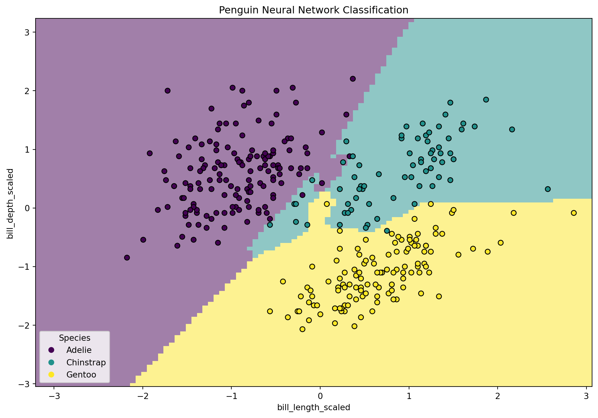
Visualizing Decision Boundary with seaborn and matplotlib

from sklearn.inspection import DecisionBoundaryDisplay
from sklearn.preprocessing import LabelEncoder

# Encode labels for plotting
label_encoder = LabelEncoder()
y_encoded = label_encoder.fit_transform(y)

# Create plot objects
fig, ax = plt.subplots(figsize=(12, 8))

# Plot decision boundary using the neural net classifier
disp = DecisionBoundaryDisplay.from_estimator(
    penguin_nn,             # use the neural network classifier (sklearn-style) 🦆
    X_test,                 # must be 2-dimensional features
    response_method='predict',
    plot_method='pcolormesh',
    xlabel="bill_length_scaled",
    ylabel="bill_depth_scaled",
    shading='auto',
    alpha=0.5,
    ax=ax
)

# Overlay test points
scatter = disp.ax_.scatter(
    X_scaled[:, 0],
    X_scaled[:, 1],
    c=y_encoded,
    edgecolors='k'
)

# Add legend using class labels from the classifier
disp.ax_.legend(
    scatter.legend_elements()[0],
    penguin_nn.classes_,
    loc='lower left',
    title='Species'
)

disp.ax_.set_title("Penguin Neural Network Classification")
fig.show()

To visualize the decision boundary of the modelm we can use another sklearn class called DecisionBoundaryDisplay, which creates a display object that has matplotlib-style plotting methods.

Because we designed our classifier to match sklearn API, we are able to use sklearn’s DecisionBoundaryDisplay with our classifier without needing additional steps.

We assign our axis in the creation of our display object and use the attached .ax_. methods to create the scatter plot and legend as well as set the title.

Because we’re using this display object, we have to explicitly call fig.show() here to display the figure.

Visualizing Decision Boundary with seaborn and matplotlib

Evaluate PenguinNet performance

To check the performance of our PenguinNet classifier, we can check the accuracy score and print a classification report.
- accuracy_score and classification_report are both functions!
- They are not unique to scikit-learn classes so it makes sense for them to be functions not methods

# Evaluate neural network performance
penguin_nn_accuracy = accuracy_score(y_test, y_pred)
print(f"Neural Network Accuracy: {penguin_nn_accuracy:.2f}")
print("Classification Report: \n", classification_report(y_test, y_pred))

Neural Network Accuracy: 0.97
Classification Report: 
               precision    recall  f1-score   support

      Adelie       0.98      0.98      0.98        44
   Chinstrap       0.95      0.90      0.92        20
      Gentoo       0.97      1.00      0.99        36

    accuracy                           0.97       100
   macro avg       0.97      0.96      0.96       100
weighted avg       0.97      0.97      0.97       100

Finally, we can use the ‘accuracy_score’ and classification_report functions to check the performance of our classifier.

Make a Summary Table of Metrics for Both Models

summary_table = pd.DataFrame({
    "Metric": ["k-Means Adjusted Rand Index", "Neural Network Accuracy"],
    "Value": [kmeans_ari, penguin_nn_accuracy]
})

(
    GT(summary_table)
    .tab_header(title="Model Results Summary")
    .fmt_number(columns="Value", n_sigfig=2)
    .tab_options(table_font_size=20)
)

Model Results Summary
Metric	Value
k-Means Adjusted Rand Index	0.82
Neural Network Accuracy	0.97

Using the great_tables package, we can make a nice little summary table of our results from both mini-projects.

Key Takeaways from This Session

• Python workflows rely on object-oriented structures in addition to functions:
  Understanding the OOP paradigm makes Python a lot easier!
• Everything is an object!
• Duck Typing:
  If an object has a method, that method can be called regardless of the object type. Caveat being, make sure the arguments (if any) in the method are specified correctly for all objects!
• Python packages use common methods that make it easy to change between model types without changing a lot of code.
• We can do the same when we design our own model classes

Return to website

Intro to Python Workshops